Implementing the Izhikevich Neuron in R

The following is an implementation of the Izhikevich Neuron in R. More details can be found at Eugene Izhikevich’s webpage.

Essentially, the Izhikevich model seeks to balance realistic modeling of neuronal membrane dynamics with computational efficiency. The model is a set of coupled differential equations:

and

Where

• $v$ is a dimensionless variable representing membrane potential
• $u$ is a dimensionless variable representing membrane potential recovery
• $a$ is a dimensionless parameter representing the time scale of $u$
• $b$ is a dimensionless parameter representing the sensitivity of $u$ to subthreshold fluctuations in $v$
• $c$ is a dimensionless parameter representing the after-spike reset value of $v$ (caused by fast high-threshold $K^{+}$ conductance)
• $d$ is a dimensionless parameter representing the after-spike reset value of $u$ (caused by slow high-threshold $Na^{+}$ and $K^{+}$ conductances)
• $I$ is an externally applied current

Setting the parameters $a = 0.02$, $b = 0.2$, $c = -65$, and $d = 2$, we will generate a fast-spiking neuron simulation.

#SPECIFY PARAMETERS
nsteps     = 500 #number of time steps over which to integrate
a          = 0.02
b          = 0.2
c          = -65
d          = 2
I          = matrix(0, nrow = nsteps, ncol = 1)
I[100:400] = 6
v_res      = 30
v          = matrix(NA, nrow = nsteps, ncol = 1)
u          = matrix(NA, nrow = nsteps, ncol = 1)
v[1]       = -70
u[1]       = b * v[1]
  
 
#IZHIKEVICH NEURON FUNCTION
Izhikevich = function(v, u, a, b, c, d, I, v_res) {
  
  if (v >= v_res) {
    v = c
    u = u + d
  } else {
    dv = (0.04 * (v^2)) + (5*v) + 140 - u + I
    v = v + dv
    
    du = a * ((b*v)-u)
    u = u + du
  }
  
  
  
  return(c(v, u))
}
 
#INTEGRATION VIA THE EULER METHOD
for (i in 1:(nsteps-1)) {
  res = Izhikevich(v[i], u[i], a, b, c, d, I[i], v_res)
  
  v[i+1] = min(res[1], v_res)
  u[i+1] = res[2]
    
}
 
#PLOT
plot(seq(1, nsteps, 1), v, 
     type = 'l',
     main = "Izhikevich Neuron",
     xlab = "Time (ms)",
     ylab = "Membrane Potential (mV)")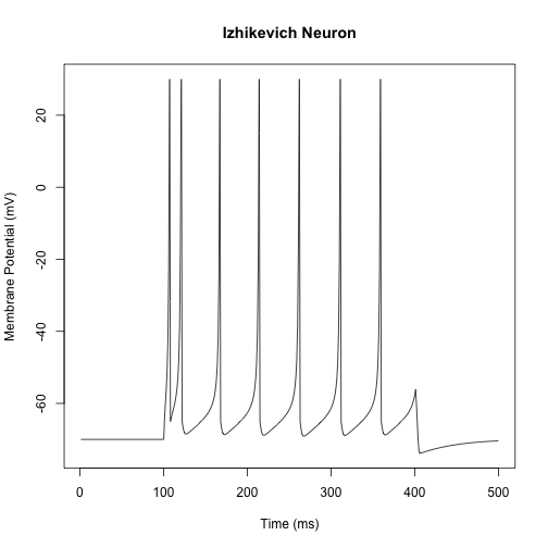

Of particular interest is that other neuron types can be simulated by adjusting the model parameters. For instance, setting the parameters $a = 0.02$, $b = 0.2$, $c = -50$, and $d = 2$ will generate a chattering neuron.

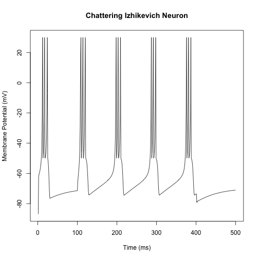
Parameters for further neuron types may be found at Eugene Izhikevich’s page (link above).