Creating Survival Curves in R
Survival analysis is a common procedure in biostatistics. Fortunately, R has extensive packages supporting these methods, including survival and KMsurv.
Generating Data
First, let’s load the packages and generate a dataframe with two dates, one for a hypothetical intervention date, and a second for an event or censoring date. The number of patients will be n = 2000.
library(survival)
library(KMsurv)

#set origin date
originDate = as.Date("2000-01-01", format = "%Y-%m-%d")

#generate random number of days to add to the origin for each patient
nDays = rnorm(2000, mean = 60, sd = 100)

#generate vector of intervention dates by adding the nDays to the origin
interventionDate = originDate + nDays

#generate vector of event dates by adding nDays to the interventionDate
#   we will add the absolute number of nDays since event must occur after intervention
eventDate = interventionDate + abs(nDays)

#generate vector of events (TRUE or FALSE)
#   TRUE represents the event of interest
#   FALSE represents a censored value
#   We will set the probability of a TRUE event (vs. censoring) to 0.95
eventType = (rbinom(2000, 1, prob = 0.95) == 1)

#put these into a dataframe
kmdf = data.frame(intervention_date = interventionDate,
                  event_date = eventDate,
                  event = eventType)
The resulting data frame will appear as follows:
##   intervention_date event_date event
## 1        1999-07-13 2000-01-01  TRUE
## 2        2000-06-03 2000-11-05  TRUE
## 3        2000-01-20 2000-02-09 FALSE
## 4        2000-02-20 2000-04-10  TRUE
## 5        2000-05-21 2000-10-09  TRUE
## 6        2000-04-26 2000-08-20  TRUE
To generate a survival object, though, we need to take the difference between the event_date and the origin_date. (We merely generated the dates above to facilitate learning how to take the difference between dates). The difference between dates can be taken as follows:
kmdf$time_to_event = as.numeric(difftime(kmdf$event_date,
                                         kmdf$intervention_date,
                                         units = "days"))
Fitting and Plotting the Survival Model
Now we will fit a survival model with a constant.
sfit = survfit(Surv(kmdf$time_to_event, kmdf$event) ~ 0)

#plot sfit

plot(sfit,
     main = "Survival Curve for Randomly Generated Data",
     xlab = "Time to Event (Days)",
     ylab = "Proportion Surviving")
Plotting Survival Curves for Multiple Groups
What about the (common) case in which there are multiple groups?
Let’s start by generating another group of n = 2000 patients whose survival is longer, but with a greater standard deviation.
#generate random number of days to add to the origin for each patient
nDaysGroup2 = rnorm(2000, mean = 200, sd = 200)

#generate vector of intervention dates by adding the nDays to the origin
interventionDateGroup2 = originDate + nDays

#generate vector of event dates by adding nDays to the interventionDate
#   we will add the absolute number of nDays since event must occur after intervention
eventDateGroup2 = interventionDateGroup2 + abs(nDaysGroup2)

#generate vector of events (TRUE or FALSE)
#   TRUE represents the event of interest
#   FALSE represents a censored value
#   We will set the probability of a TRUE event (vs. censoring) to 0.95
eventTypeGroup2 = (rbinom(2000, 1, prob = 0.95) == 1)

#put these into a dataframe
kmdfGroup2 = data.frame(intervention_date = interventionDateGroup2,
                        event_date = eventDateGroup2,
                        event = eventTypeGroup2)

#compute time to event for new data frame
kmdfGroup2$time_to_event = as.numeric(difftime(kmdfGroup2$event_date,
                                               kmdfGroup2$intervention_date,
                                               units = "days"))
We’ll need to bind the two data frames together, so we’ll add a column to indicate the group names to each data frame before we stick them together.
kmdf$group       = "Control"
kmdfGroup2$group = "Treatment"


kmdf_2groups = rbind(kmdf, kmdfGroup2)
We’ll now generate and plot the survival model as before, with the new data frame kmdf_2groups. Note, however, that the term which was formerly constant is now set to the group variable of the new data frame, such that we get two survival curves (one for each group).
sfit2 = survfit(Surv(kmdf_2groups$time_to_event, kmdf_2groups$event) ~ kmdf_2groups$group)

#plot sfit

plot(sfit2,
     main = "Survival Curve for Two Groups of Randomly Generated Data",
     xlab = "Time to Event (Days)",
     ylab = "Proportion Surviving",
     col  = c(1, 2))

legend("topright",
       levels(factor(kmdf_2groups$group)),
       col = c(1,2),
       lty = 1)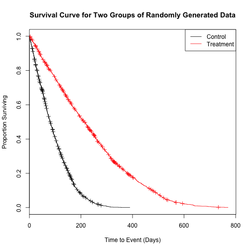
Conclusion
Generating survival curves in R is very simple, and can be quite rewarding (particularly if you are using a real data set).