Exploring Suicide Rates by Number of Health Care Workers Employed (or Testing a Blog Post with RStudio)
I just recently figured out how to set up a blog on GitHub and publish pages with RStudio, thereby allowing me to convert the constant stream of notes I make in .Rmd format into more than just files on my hard drive. I’ll just test out a quick one here with a look at whether the suicide rate in a country (per 100,000) will vary with the number of psychiatrists, nurses, social workers, and psychologists working in the mental health sector. I’ll use data from the WHO API.
The last available dataset for suicide rates was 2012, whereas for the healthcare professional employment rates, 2011 was the last data collection year.
We’ll begin by downloading the data.
library(dplyr)
library(caret)
library(ggplot2)
library(rworldmap)

#download suicide rate data from WHO api
code        = "MH_12"
year        = 2012
url         = paste0('http://apps.who.int/gho/athena/api/GHO/',code,'.csv?filter=COUNTRY:*;YEAR:',year)
suicideRate = read.csv(url,as.is=TRUE)

#download number of psychiatrists working in mental health sector from WHO api
code           = "MH_6"
year           = 2011
url            = paste0('http://apps.who.int/gho/athena/api/GHO/',code,'.csv?filter=COUNTRY:*;YEAR:',year)
nPsychiatrists = read.csv(url,as.is=TRUE)

#download number of nurses working in mental health sector from WHO api
code    = "MH_7"
year    = 2011
url     = paste0('http://apps.who.int/gho/athena/api/GHO/',code,'.csv?filter=COUNTRY:*;YEAR:',year)
nNurses = read.csv(url,as.is=TRUE)

#download number of social workers working in mental health sector from WHO api
code = "MH_8"
year = 2011
url  = paste0('http://apps.who.int/gho/athena/api/GHO/',code,'.csv?filter=COUNTRY:*;YEAR:',year)
nSws = read.csv(url,as.is=TRUE)

#download number of psychologists working in mental health sector from WHO api
code           = "MH_9"
year           = 2011
url            = paste0('http://apps.who.int/gho/athena/api/GHO/',code,'.csv?filter=COUNTRY:*;YEAR:',year)
nPsychologists = read.csv(url,as.is=TRUE)
Let’s have a look at some maps.
#create the suicide rate map
suicideMap = joinCountryData2Map(suicideRate,
                                 nameJoinColumn="COUNTRY",
                                 joinCode="ISO3")
FALSE 516 codes from your data successfully matched countries in the map
FALSE 0 codes from your data failed to match with a country code in the map
FALSE 72 codes from the map weren't represented in your data#map the suicide data
mapCountryData(suicideMap,
nameColumnToPlot="Numeric",
catMethod="fixedWidth",
mapRegion="world",
mapTitle="Suicide Rates per 100,000",
colourPalette = "negpos8")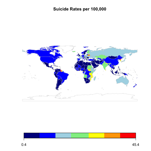
#-----------------------------------------------------------------

#create the psychiatrist distribution map
psychiatristMap = joinCountryData2Map(nPsychiatrists,
                                      nameJoinColumn="COUNTRY",
                                      joinCode="ISO3")
FALSE 180 codes from your data successfully matched countries in the map
FALSE 0 codes from your data failed to match with a country code in the map
FALSE 64 codes from the map weren't represented in your data#map the psychiatrist data
mapCountryData(psychiatristMap,
nameColumnToPlot="Numeric",
catMethod="fixedWidth",
mapRegion="world",
mapTitle="Number of Psychiatrists per 100,000",
colourPalette = "negpos8")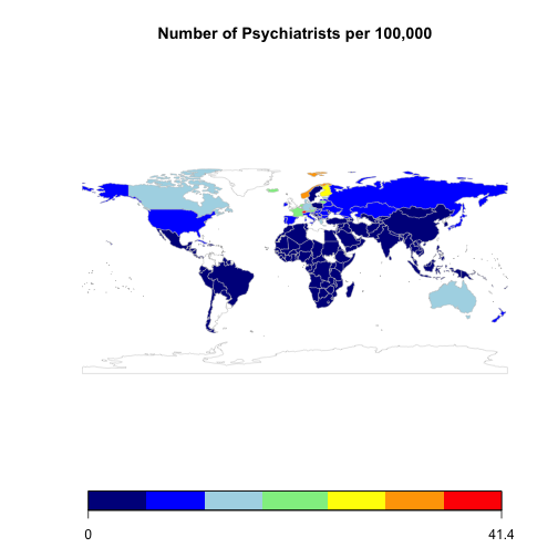
#-----------------------------------------------------------------

#create the nurse distribution map
nurseMap = joinCountryData2Map(nNurses,
                               nameJoinColumn="COUNTRY",
                               joinCode="ISO3")
FALSE 163 codes from your data successfully matched countries in the map
FALSE 0 codes from your data failed to match with a country code in the map
FALSE 81 codes from the map weren't represented in your data#map the nurse data
mapCountryData(nurseMap,
nameColumnToPlot="Numeric",
catMethod="fixedWidth",
mapRegion="world",
mapTitle="Number of Mental Health Nurses per 100,000",
colourPalette = "negpos8")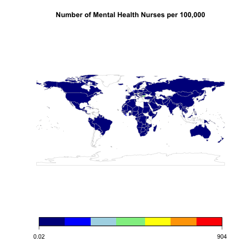
#-----------------------------------------------------------------

#create the social worker distribution map
swMap = joinCountryData2Map(nSws,
                            nameJoinColumn="COUNTRY",
                            joinCode="ISO3")
FALSE 138 codes from your data successfully matched countries in the map
FALSE 0 codes from your data failed to match with a country code in the map
FALSE 106 codes from the map weren't represented in your data#map the socal worker data
mapCountryData(swMap,
nameColumnToPlot="Numeric",
catMethod="fixedWidth",
mapRegion="world",
mapTitle="Number of Mental Health Social Workers per 100,000",
colourPalette = "negpos8")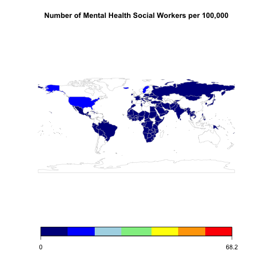
#-----------------------------------------------------------------

#create the psychologist distribution map
psychologistMap = joinCountryData2Map(nPsychologists,
                                      nameJoinColumn="COUNTRY",
                                      joinCode="ISO3")
FALSE 156 codes from your data successfully matched countries in the map
FALSE 0 codes from your data failed to match with a country code in the map
FALSE 88 codes from the map weren't represented in your data#map the psychiatrist data
mapCountryData(psychologistMap,
nameColumnToPlot="Numeric",
catMethod="fixedWidth",
mapRegion="world",
mapTitle="Number of Psychologists per 100,000",
colourPalette = "negpos8")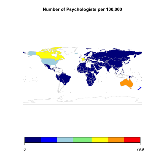
Next, we’ll merge them into a single data frame.
#add additional column to account for for "SEX" column of suicideRate
nNurses$SEX        = NA
nPsychiatrists$SEX = NA
nPsychologists$SEX = NA
nSws$SEX           = NA

#rbind and cast the data frames
dataMerged     = rbind(suicideRate[suicideRate$SEX == "BTSX",], nPsychiatrists)
dataMerged     = rbind(dataMerged, nPsychologists)
dataMerged     = rbind(dataMerged, nSws)
dataMerged     = rbind(dataMerged, nNurses)

dataMergedCast = dcast(data = dataMerged, REGION + COUNTRY ~ GHO, value.var = "Numeric")

#rename
names(dataMergedCast) = c("region",
                          "country",
                          "suicide_rate",
                          "n_psychiatrists",
                          "n_nurses",
                          "n_social_workers",
                          "n_psychologists")

#plot unnormalized
ggplot(dataMergedCast, aes(x = suicide_rate)) +
  geom_density(aes(fill = region), alpha = 0.2) +
  ggtitle("Suicide Rate per 100,000 Across Countries") +
  xlab("Suicide Rate per 100,000") +
  theme_classic()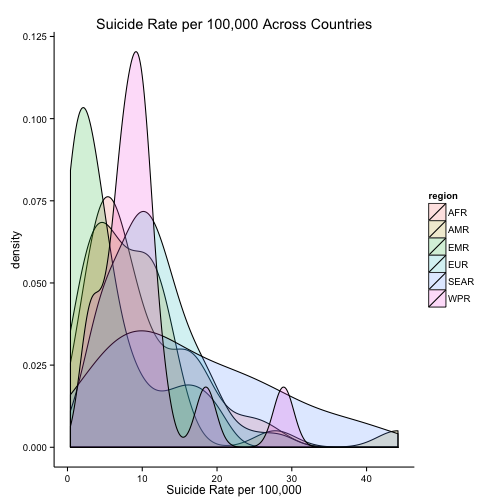
ggplot(dataMergedCast, aes(x = log(n_psychiatrists))) +
  geom_density(aes(fill = region), alpha = 0.2) +
  ggtitle("Psychiatrists per 100,000 Across Countries") +
  xlab("Log Number of Psychiatrists per 100,000") +
  theme_classic()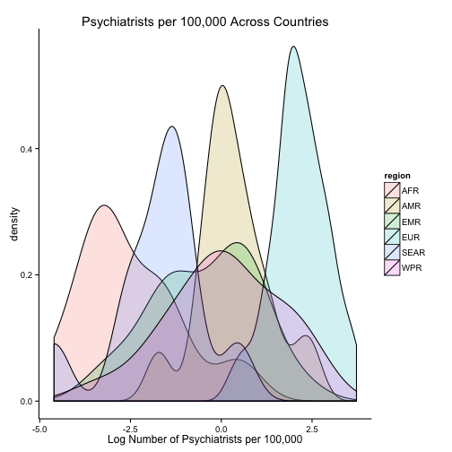
ggplot(dataMergedCast, aes(x = log(n_nurses))) +
  geom_density(aes(fill = region), alpha = 0.2) +
  ggtitle("Nurses per 100,000 Across Countries") +
  xlab("Log Number of Nurses per 100,000") +
  theme_classic()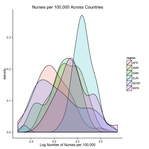
ggplot(dataMergedCast, aes(x = log(n_social_workers))) +
  geom_density(aes(fill = region), alpha = 0.2) +
  ggtitle("Social Workers per 100,000 Across Countries") +
  xlab("Log Number of Social Workers per 100,000") +
  theme_classic()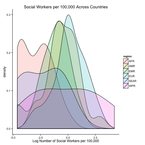
ggplot(dataMergedCast, aes(x = log(n_psychologists))) +
  geom_density(aes(fill = region), alpha = 0.2) +
  ggtitle("Psychologists per 100,000 Across Countries") +
  xlab("Log Number of Psychologists per 100,000") +
  theme_classic()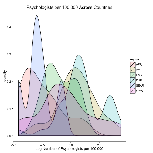
#normalize variables
dataMergedCastNorm = dataMergedCast
for (i in 3:7) {
  dataMergedCastNorm[,i] = (dataMergedCastNorm[,i] - mean(dataMergedCastNorm[,i], na.rm = TRUE))/sd(dataMergedCastNorm[,i], na.rm = TRUE)
}

#create plots

ggplot(dataMergedCastNorm, aes(x = reorder(country, suicide_rate), y = suicide_rate)) +
  geom_bar(stat = "identity", aes(fill = region)) +
  coord_flip() +
  ggtitle("Suicide Rate per 100,000 Across Countries") +
  xlab("Country") +
  ylab("Normalized Suicide Rate per 100,000") +
  theme_classic() +
  theme(axis.text.y = element_text(vjust = 1, hjust = 1))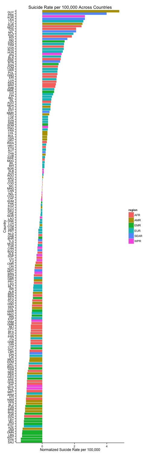
ggplot(dataMergedCastNorm, aes(x = log(n_psychiatrists), y = suicide_rate)) +
  geom_point(aes(colour = region)) +
  geom_smooth(method = "lm") +
  ggtitle("Suicide Rate by Number of Psychiatrists per 100,000") +
  xlab("Log Normalized Number of Psychiatrists per 100,000") +
  ylab("Normalized Suicide Rate per 100,000") +
  theme_classic()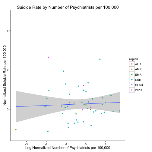
ggplot(dataMergedCastNorm, aes(x = log(n_nurses), y = suicide_rate)) +
  geom_point(aes(colour = region)) +
  geom_smooth(method = "lm") +
  ggtitle("Suicide Rate by Number of Nurses per 100,000") +
  xlab("Log Normalized Number of Nurses per 100,000") +
  ylab("Normalized Suicide Rate per 100,000") +
  theme_classic()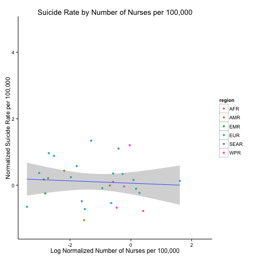
ggplot(dataMergedCastNorm, aes(x = log(n_social_workers), y = suicide_rate)) +
  geom_point(aes(colour = region)) +
  geom_smooth(method = "lm") +
  ggtitle("Suicide Rate by Number of Social Workers per 100,000") +
  xlab("Log Normalized Number of Social Workers per 100,000") +
  ylab("Normalized Suicide Rate per 100,000") +
  theme_classic()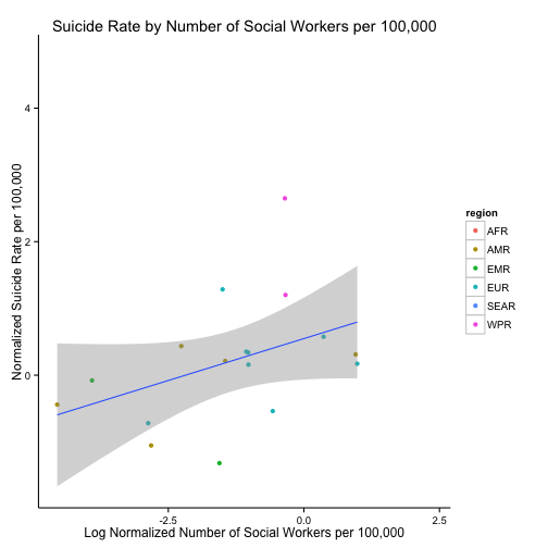
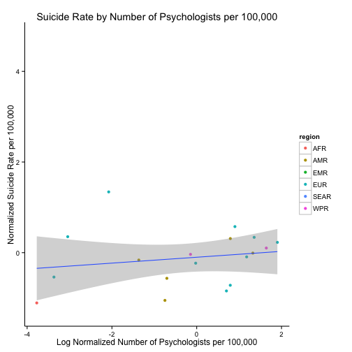
ggplot(dataMergedCastNorm, aes(x = log(n_psychologists), y = suicide_rate)) +
  geom_point(aes(colour = region)) +
  geom_smooth(method = "lm") +
  ggtitle("Suicide Rate by Number of Psychologists per 100,000") +
  xlab("Log Normalized Number of Psychologists per 100,000") +
  ylab("Normalized Suicide Rate per 100,000") +
  theme_classic()